A free DLC for the {lubridate} package which makes it fast and easy to perform set operations (e.g. intersection, union, set-difference) on datetime intervals. Disclaimer, I am not affiliated with {lubridate}!
Published
January 30, 2025
{lubridate} is Great
I love {lubridate} because I do not love working with dates - or their malicious cousins, times. This is probably a cliché among people who think about data for a living, but I will reiterate it anyway; I don’t like thinking about time zones, leap years, how many days are in April, or dealing with base-60 arithmetic.
Fortunately, {lubridate} provides a collection of datetime classes and functions which, more often than not, keep me safely within a bubble where I don’t need to think about these things. If you’re unfamiliar with {lubridate}, here are a few examples.
library(lubridate, warn.conflicts =FALSE)dyears(1) /dminutes() # How many minutes are in an average year?
[1] 525960
ddays(366) /dminutes() # How many minutes are in a leap year?
[1] 527040
# Convert a UTC datetime to an EST datetimewith_tz(ymd_hms("2012-03-26 10:10:00", tz ="UTC"), "EST")
[1] "2012-03-26 05:10:00 EST"
There is, however, one family of problems that {lubridate} does not like. Problems with holes. Consider work and lunch, which measure the time-spans I spent at work and on a lunch break on January 3rd 2025.
work <-interval("2025-01-03 09:00:00", "2025-01-03 17:00:00")lunch <-interval("2025-01-03 12:00:00", "2025-01-03 13:00:00")
What I’d like to analyze is the time that I was actually doing work, excluding my lunch break. My first instinct is to punch a hole through my work day using setdiff() to remove the time I spent at lunch. Unfortunately for me, this isn’t going to work.
try(setdiff(work, lunch))
Error in setdiff.Interval(work, lunch) :
  Cases 1 result in discontinuous intervals.
The phrase “discontinuous intervals” here is a fancier way of saying “holey intervals”.
Holey Intervals
A <phinterval> is a “potentially-holey-interval” vector, i.e. it’s an interval which might contain gaps. In particular, each element of a <phinterval> vector is a set of non-overlapping, non-abutting datetime intervals.
<phinterval<UTC>[1]>
[1] [2020-01-07--2020-01-08, 2020-01-09--2020-01-12] UTC
A few things of note about the <phinterval> vector phint:
The element phint[[1]] describes two non-overlapping time spans.
phint[[1]] contains a “hole” during January the 8th.
When creating phint, phinterval() combined jan_9_to_10 and jan_9_to_12.
Many date and time related concepts are naturally represented by a <phinterval>, including which portion of the day was I actually working on January 3rd, 2025.
phint_diff(work, lunch)
<phinterval<UTC>[1]>
[1] [2025-01-03 09:00:00--2025-01-03 12:00:00, 2025-01-03 13:00:00--2025-01-03 17:00:00] UTC
Hard Questions with Dates
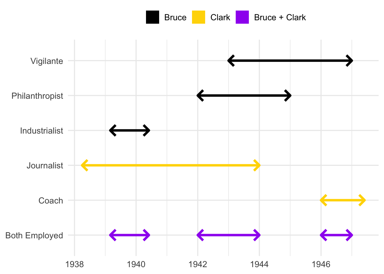
To further motivate the existence of a <phinterval>, lets consider a fake employment dataset. We’ll pretend that we’re government employees who’ve been tasked with analyzing the employment history of respondents to the latest census survey. Each person who responded to the census provided us with the title and start/end date of every job they’ve ever held.
print(employment)
# A tibble: 9 × 3
name job_title job_interval
<chr> <chr> <Interval>
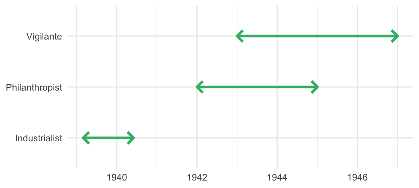
1 Bruce Industrialist 1939-03-01 UTC--1940-06-01 UTC
2 Bruce Philanthropist 1942-01-01 UTC--1945-01-01 UTC
3 Bruce Vigilante 1943-01-01 UTC--1947-01-01 UTC
4 Clark Journalist 1938-04-01 UTC--1944-01-01 UTC
5 Clark Coach 1946-01-01 UTC--1947-06-01 UTC
6 Tony Inventor 1962-12-01 UTC--1963-06-01 UTC
7 Tony CEO 1964-01-01 UTC--1967-01-01 UTC
8 Tony Consultant 1966-01-01 UTC--1967-01-01 UTC
9 Natasha Spy 1964-04-01 UTC--1970-01-01 UTC
Our boss has a few questions for us:
When was each respondent employed?
When did each respondent have gaps in their employment?
We’ll focus on "Bruce" first. Our office uses the {tidyverse}, so we’ll be working with {dplyr}, {ggplot2}, and {lubridate}.
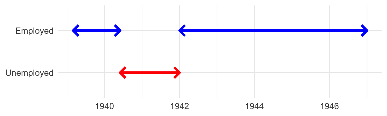
To answer our boss’s first question, we’re looking to find the blue time-spans where Bruce was employed. This is surprisingly un-simple. Here’s a handful of Stack Overflow posts with tens of thousands of views between them asking how to do exactly this:
Answers to these questions suggest using packages ranging from {data.table} to {IRanges} to {ivs}. Here’s a fast-ish solution using {base} R.
# Extract the start and end of each of Bruce's jobsintervals <-sort(bruce_employment$job_interval)starts <-int_start(intervals)ends <-int_end(intervals)# Do some magic to merge overlapping jobsoverlap_groups <-c(0, cumsum(as.numeric(lead(starts)) >cummax(as.numeric(ends)))[-length(ends)])new_starts <-do.call(c, split(starts, overlap_groups) |>lapply(min))new_ends <-do.call(c, split(ends, overlap_groups) |>lapply(max))# Turn this back into an <Interval> vectorbruce_employment_intervals <-interval(new_starts, new_ends)print(bruce_employment_intervals)
[1] 1939-03-01 UTC--1940-06-01 UTC 1942-01-01 UTC--1947-01-01 UTC
Suffice it to say, we’ve firmly left the warm embrace of {lubridate}’s intuitive API. To answer our boss’s second question, when was Bruce unemployed between jobs, we perform another slightly less confusing dance.
# Extract the start and end of each of Bruce's employment spansstarts <-int_start(bruce_employment_intervals)ends <-int_end(bruce_employment_intervals)# Turn the ends of employment into the starts of unemploymentbruce_unemployment_intervals <-interval(ends[-length(ends)], starts[-1])print(bruce_unemployment_intervals)
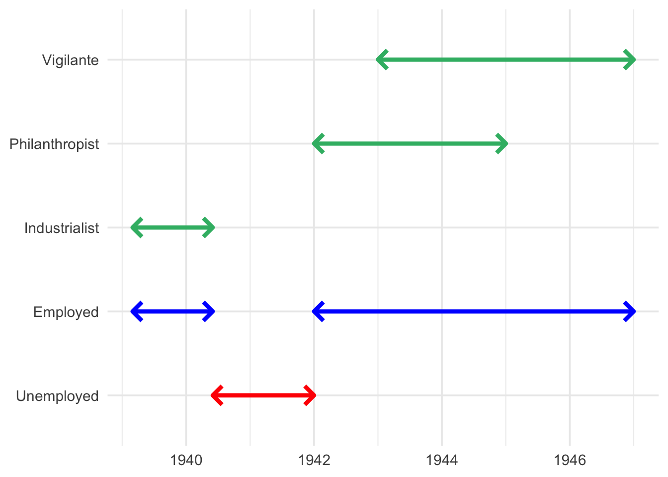
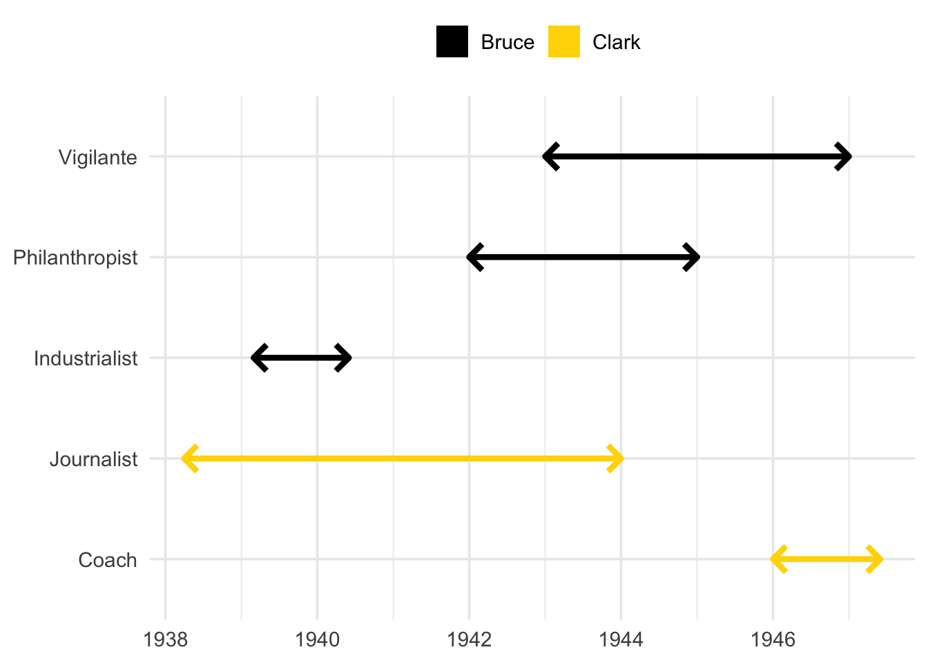
We present this plot to our boss. They look at us, perplexed, and ask why it took 30 minutes to make this one image. Anyhow, they grumble, for our next task we need to find all periods where Bruce and Clark were working at the same time.
I’m going to spare you the details of how we’d do this, but it’s not fun. And the questions only get more complicated from here.
Enter {phinterval}
The goal of the {phinterval} package is to ever-so-slightly expand the bubble that {lubridate} created, so that we can solve problems like these using a familiar API. The <phinterval> vector class and it’s methods are designed to look right at home alongside the classes implemented by {lubridate}:
<Duration> - A length of time in seconds.
<Period> - A length of time in minutes, hours, days, weeks, months, or years.
<Interval> - A span of time between two instants.
<phinterval> - An <Interval> which may contain holes.
Returning to our boss’s first request, what we’re really trying to do is flatten/merge/combine an <Interval> vector into a <phinterval> element. We can do this via phint_squash() which squashes an <Interval> vector into a scalar <phinterval>.
<phinterval<UTC>[1]>
[1] [1939-03-01--1940-06-01, 1942-01-01--1947-01-01] UTC
For our boss’s second request, we just want to retrieve the “holes” of our <phinterval> which represent the gaps in Bruce’s employment. We can do this using phint_invert() which returns the gaps of an existing <phinterval> vector as a new <phinterval>.
phint_invert(bruce_employed)
<phinterval<UTC>[1]>
[1] [1940-06-01--1942-01-01] UTC
{phinterval} really starts to shine when we use it alongside {dplyr}.
# A tibble: 4 × 3
  name                                                employed
  <chr>                                             <phintrvl>
1 Bruce   [1939-03-01--1940-06-01, 1942-01-01--1947-01-01] UTC
2 Clark   [1938-04-01--1944-01-01, 1946-01-01--1947-06-01] UTC
3 Natasha                         [1964-04-01--1970-01-01] UTC
4 Tony    [1962-12-01--1963-06-01, 1964-01-01--1967-01-01] UTC
# ℹ 1 more variable: unemployed <phintrvl>
Our boss’s intimidating third question is now just a matter of taking the intersection of Bruce’s and Clark’s employment histories with phint_intersect().
Unfortunately, while all of the code in this demo works, {phinterval} is still a prototype. Because of it’s non-standard data-structure, we can’t just use fast vectorized operators or primitive functions when manipulating a <phinterval>’s data. Looking at the source code for the <phinterval> class you’ll see a liberal use of map(), a wrapper around base::lapply().
This is slow, sometimes very slow. Compare the function body of lubridate::int_end(), which retrieves the end time of an <Interval>, with the function body of phinterval::phint_end(), which retrieves the end time of a <phinterval>.
{phinterval}, relatively speaking, is doing a lot of work to accomplish a pretty simple task. To improve performance, I’d like to implement a portion of the {phinterval} package in C++ (with the help of the {Rcpp} package) and work on optimizing the remaining R code.
Until then, if you need fast and flexible interval operations, I’d recommend Davis Vaughn’s great {ivs} package. It can do anything shown in this article and it’s powered by fast {vctrs} functions already written in C++.
Why {phinterval}
If {ivs} works, why bother with {phinterval}? First, because writing new packages is fun. Second, because {ivs}, by design, is not meant to be an extension of the <Interval> vector (an <ivs_iv> can represent a right-open interval of any vector type which has methods for comparison and is supported by the {vctrs} package).
{phinterval}, meanwhile, is designed to be a drop-in extension of the {lubridate} package. If you’re lucky, and your boss doesn’t ask too many questions, you’ll never need it. If you’re less lucky, you can take solace in the fact that you shouldn’t need to change any of your existing {lubridate} work-flow to start working with {phinterval}. Any {lubridate} <Interval> vector can be coerced to an equivalent <phinterval> vector without loss of information, including instantaneous intervals. <phinterval> vectors also support many of the useful features of an <Interval>, including date arithmetic and coercion to a duration or period.
Users of {lubridate} will already know how to use many of the phint_*() family of functions, all of which accept an <Interval> or <phinterval> vector as input.
{lubridate}
{phinterval}
Returns
int_length()
phint_length()
Length in seconds
int_start()
phint_start()
Start date of the (ph)interval
int_end()
phint_end()
End date of the (ph)interval
int_shift()
phint_end()
A (ph)interval shifted up/down the timeline
int_overlaps()
phint_overlaps()
Whether elements of two ph(intervals) overlap
%within%
%within%
Whether a (ph)interval is within another ph(interval)
When you do need to reach for the unique functionality of {phinterval}, functions such as phint_union(), phint_intersection(), and phint_diff() all accept any <Interval> vector as input and output a <phinterval> vector with the same timezone.